In which computers tell the difference between space and medicine

January 01, 2016 | 13 Minute Read

Machine Learning is both awesome and popular in both research and industry. However, I haven’t found many introductory tutorials on it that combine math and implementation. So, in this blog post I hope to do both by showing how to use the perceptron learning algorithm to classify articles by topic.

If you want to follow along with the code, clone akornilo/perceptron-learning.git. You will only need Python to run it.

The data

The data we will be classifying is part of the 20 newsgroups dataset and consists of online articles on various topics. The data we will be using has been tranformed in several ways:

Each article has been transformed into a dictionary mapping words to how many times they appear in the article.
The articles have been grouped into pairs of similar topics: macintosh vs ibm, medical vs space, and atheist vs christian.

Although, these changes sacrifice some of the information, they make it simple for us to dive into the classification task. You can check out the data in the ‘data’ subdirectory of the github repo. For each pair of topics, there are four files: *.dev, *.test, *.train and *.response. The dev, test and train files contain the split up data, with lines of the format (this example is from the medspace.train file):

60801.s	{"control": 2, "in": 1, "au": 1, "thanks": 1, "edu": 1, "cold": 2, "sounding": 1, "size": 1, "from": 1, "for": 1, "how": 1, "jim": 1, "anyone": 1, "to": 1, "does": 1, "subject": 1, "roll": 2, "8725157m": 1, "australia": 1, "thruster": 2, "gas": 2, "levels": 1, "know": 1, "tanks": 2, "<digit>": 1, "advance": 1, "of": 1, "university": 1, "lines": 1, "unisa": 1, "rockets": 1, "organization": 1, "south": 1}

where the first value is the id of the article and the second is its content. The response file has lines of the format:

 51762.s	0

with the first value representing the article, and the second (a 0 or a 1) representing its category.

The algorithm

The perceptron learning algorithm (PLA) attempts to classify data between two categories by trying to find a hyperplane that separates the categories. This is a simple example showing a possible solution line (hyperplane of 2 dimensions) that PLA could find:

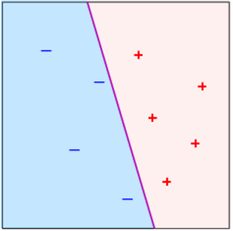
For our example, we will take each word to be a dimension, and the number of times it appears as the corresponding value. Thus, each article can be thought of as a vector of the length of all the words in all the articles with zeroes in most dimensions.

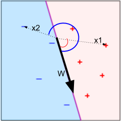
The hyperplane is represented by a “weight vector” w. To classify an article (represented by vector x), we look at:

The sign will tell us which side of the hyperplane the article belongs on, and consequently which category it is in. This method works because the dot product is equal to the product of the magnitudes of the two vectors and the cosine of the angle between them:

Since magnitudes are always non-negative, the sign is determined by the cosine which will be positive for angles between 0 and 180 and negative for the rest:

Since given a weight vector we can classify any article, the goal of the algorithm is to find this vector.

Finding “w”

A good weight vector will be one that classifies most of the training data correctly. One way to capture this criteria is by using a loss function which represents how much of the data is misclassified. The perceptron loss function is defined as follows (x represents the vector for a training data point, y represents the label (1 or -1) and ‘N’ is the total number of training data points):

If the weight vector classified a point correctly, then

and the max will be 0, otherwise the max will represent the “distance” in the wrong direction.

To find a good weight vector, we should minimize this loss function. One way to do it is with stochastic gradient descent. This method iteratively considers the training points, finds the loss using the weights at the time, then finds the gradient of the loss function and moves against it. Since the gradient represents the direction of greatest increase, moving in the opposite direction will minimize the loss the most.

When we are looking at some point i, the loss is:

The gradient (derivative with respect to the weights) of this loss is:

This leads to the update rule for the weights:

which is how PLA is usually presented. Put together the algorithm is:

w = (0,0....,0) #Initialize the weights
For training points x_1...x_n:
	v_i = w * x_i # Predict the label
	if y_i * v_i < 0: # Predicted wrong
		w = w + y_i * x_i

The code

Now that we have come up with the algorithm, let’s implement it and classify our articles! The code is avalible in the perceptron.py file in the github repo. You can run it from the repository with:

python perceptron.py

Lines 1 - 37 contain set-up code for the data. Next, we represent our vectors use python dictionaries (essentially maps from keys to values) which map words to an integer. This allows us to only store non-zero values, which is important given how sparse word vectors are. Lines 39-50 have two helper functions to deal with this unusual representation:

def dotProd(v1, v2):
	total = 0
	for key, val in v1.items():
		total += val * v2.get(key, 0)
	return total

def vecAdd(v1, v2, sign = 1):
	for key, val in v2.items():
		v1[key] = v1.get(key, 0) + sign * val
	return v1

With this set-up, we are ready to run the algorithm. First, we initialize the weights to zero (with an empty dictionary).

weights = {}

Next, we run the update procedure over the training data points:

# Pick a fixed number of times to iterate through the data
for i in range(10):
	# Shuffle points to avoid bias in presentation
	shuffle(points)

	for article, vec in points:

		dp = dotProd(weights, vec)

		actualSign = key[article]

		# Check if article was misclassified
		if not (dp * actualSign > 0):
			weights = vecAdd(weights, vec, actualSign)

The first four lines may look a little unusual, but they serve two purposes. First, given a limited number of points, we can use them multiple times to come up with a better boundary. Second, by shuffling the points, we avoid potential biases with how the data is presented. Finally, I chose to use 10 iterations because I experimentally found this value to lead to a consistent performance (for more details, see convergence section at the end of the article). The rest of the lines follow the update procedure that we derived mathematically.

Finally, we evaluate the performance on both the train and the test data. Although, more sophisticated procedures evaluation methods exist, for now let’s just see how many points we classified incorrectly:

def evalData(weights, points):
	global key
	wrong = 0

	for article, vec in points:

		dp = dotProd(weights, vec)

		actualSign = key[article]

		# Check if article was misclassified
		if not (dp * actualSign > 0):
			wrong += 1
	return wrong

wrong = evalData(weights, trainData)
total = len(trainData)
print "Train Data:", wrong, total, wrong * 100.0 / total

testData = parseDataFile("data/" + category + ".test").items()
wrong = evalData(weights, testData)
total = len(testData)
print "Test data:", wrong, total, wrong * 100.0 / totall

With this code (under 100 lines!), we are ready to train and test our model!

Results

Our data set has three pairs of categories. The pair that the code is run on can be modified in line 4. These are the results for each of the pairs (because of the shuffle, your results may differ slightly):

Medical vs Space articles

Train Data: 0 952 0.0
Test data: 45 790 5.69620253165

Mac vs IBM

Train Data: 0 929 0.0
Test data: 108 777 13.8996138996

Atheist vs Christian

Train Data: 0 870 0.0
Test data: 65 717 9.06555090656

Overall, we get a great performance - we were able to classify the training data perfectly and over 86% of the test data correctly. To understand why the algorithm performs so well, let’s consider the weights. These were the terms with the heaviest weights for the space and medical categories:

Medical: mwra, dept, doctor, disease, city, medical, what, health, his, scientific

Space: space, c, orbit, earth, nasa, moon, jupiter, dc, part, just

Some of these terms make a lot of sense and follow the same cues humans would use (words like space or moon generally appear in articles about space not medicine). Other terms are a bit surprising, like ‘what’ in medical or ‘part’ in space; these may either represent idiosyncrasies of the particular dataset or true subconcious trends of writing in these areas. In the first case, these weights may lead to overfitting (see section below); in the later, they provide insight about subconcious human patterns. Given the limited training data, it is hard to tell which is the case. Overall, its pretty cool that even a simple algorithm can find the same cues as humans. The weights for the other categories show similar patterns:

Mac: mac, apple, quadra, centris, powerbook, macintosh, gnd, iisi, kemper, macs

IBM: dos, pc, off, gateway, ide, controller, windows, drives, mode, bus

Atheist: nntp, host, postings, article, x, re, atheists, atheism, writes, de, thoughts

Christian: rutgers, athos, christians, our, who, christ, will, god, heaven, question

What’s next

Our implementation gave us a pretty good results, but it also highlighted a couple of important (and common) issues.

Overfitting

As you may have noticed, the final weight vector performed much better on the training data (that was used to create it) than the test data. This phenomenon is known as overfitting; it occurs when we find a weight vector which represents the training data very well, but does not generalize beyond it. Two common solutions are reguralization and cross-validation (I may expand the code to involve these in later posts).

Linear separability

PLA makes the assumption that all the data can be separated by a hyperplane (as shown in the image above). In reality data may look more like this:

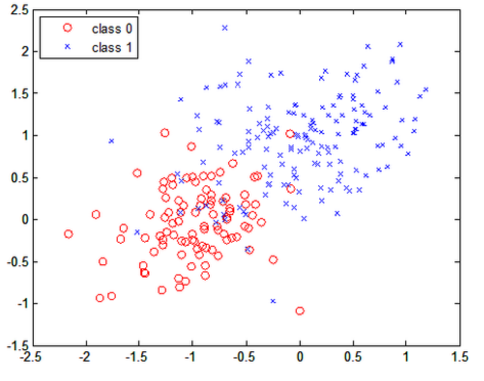
Although our training data was linearly separable because we were able to find a hyperplane that classified all the articles correctly, it did not generalize to our test data. Approaches to resolve non-linearly separable data include the voting perceptron (found on page 19 here) and kernels.

Convergence

A common problem with machine learning algorithms is to know when to stop because you’ve found the optimal solution. If the data was linearly separable, PLA will converge to a solution (you can find the proof on page 13 here). Although, there exist methods to tell when you have converged, in our case running the code a fixed number of iterations is sufficient (I experimented with several values to find one that worked well). The downside of using a finite number of iterations is that the final weight vector may not be optimal - running the code several times, I got varying levels of performance on the test data: for the medical vs space, percent incorrect varied between 5 and 8 percent; for mac vs ibm between 13 and 15 percent; for atheist vs christian between 7 and 10 percent.

This happens because many different hyperplanes separate the training data perfectly. To pick between these solutions, we will need to turn to support vector machines!! I may cover these extensions in more detail later, but, for now I hope this post will help you dive deeper into this exciting area of research. :)

Image Sources:

Links in article:

« A brief introduction to computational semantics How to ask a question (automatically) »

Anaphora Resolved